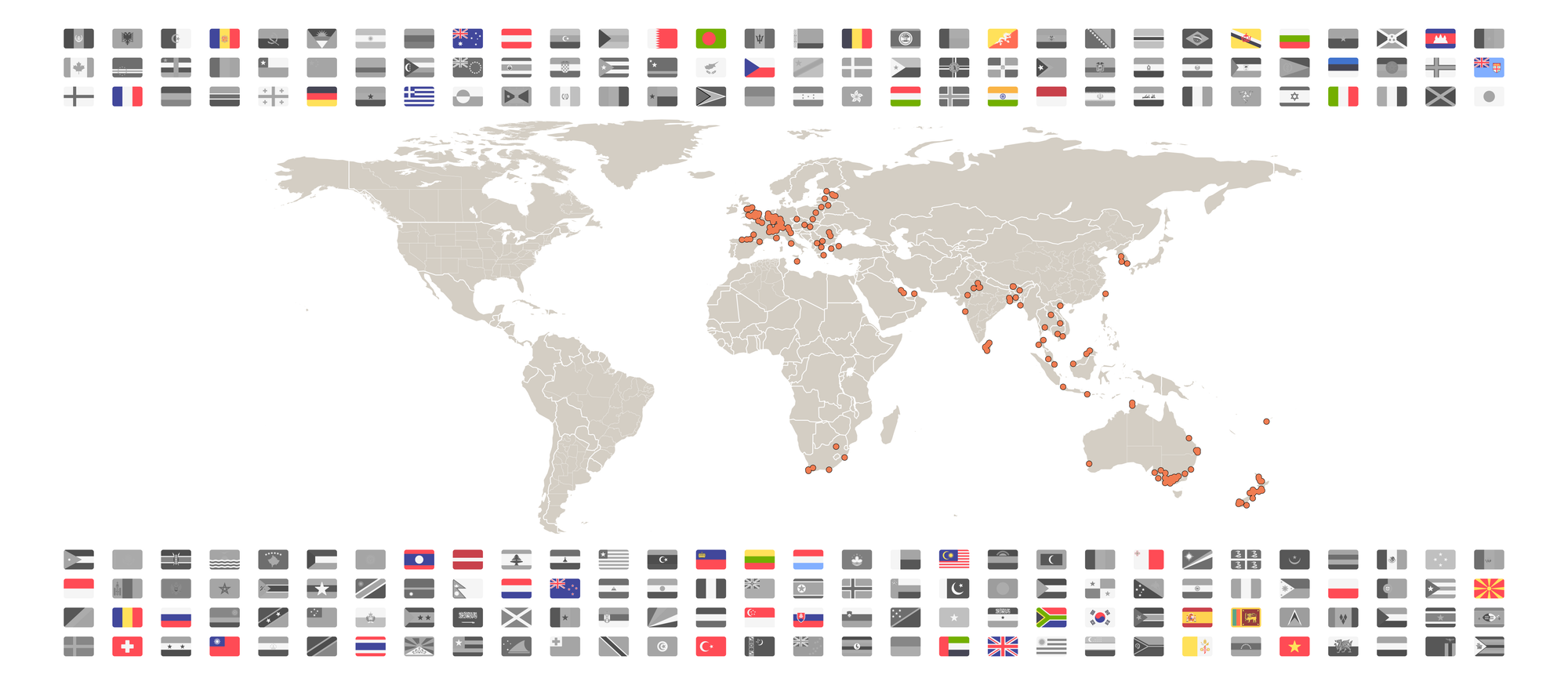
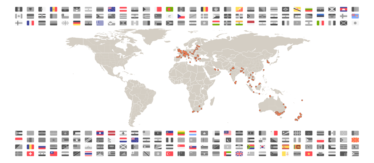
How to build a travel map in R (Updated 2025)
One of my first posts on this site was how to create a travel map in R. I always wanted to re-visit that map to add new destinations, to make the code more efficient, to use better packages.
In the old map, I found that the grouping by continent was a lot of coding effort for not much pay-off, alphabetical sorting would be easier and intuitive to readers. I also wanted to write the greying out unvisited countries into the code itself instead of photoshopping the flags manually. There were a lot of changes to make.
After much delay, I finally got around to doing just that! Here's the updated map, and if you want to create your own map like this in R you can take the code below and adapt it to your travels.

Code
Setup
pacman::p_load(
  char = c(
    "googlesheets4",
    "rnaturalearth",
    "countrycode",
    "tidyverse", # For everything
    "patchwork", # For better plot layout
    "rappdirs",
    "ggimage",  # For images on plots
    "giscoR",
    "magick",
    "rvest",
    "here",
    "sf",
    "fs"
    )
  )

graph_colours <- c(
  "Visited"        = "#F07C51",
  "Planned"        = "#FFCF66",
  "Travel_outline" = "#000000",
  "Country_fill"   = "#D4CEC4",
  "Border_line"    = "#FFFFFF"
  )
Read
Trips
df_trips <- googlesheets4::read_sheet(URL) %>%
  janitor::clean_names() %>%
  mutate(
    visited = if_else(status == "Visited", TRUE, FALSE),
    place_country = ifelse(
      is.na(place_country),
      paste(place, country, sep = ", "),
      place_country),
    iso2  = countrycode::countrycode(
      sourcevar = country,
      origin = "country.name",
      destination = "iso2c",
      custom_match = c(
        "Kosovo" = "XK",
        "United Kingdom" = "GB"
        )
      )
    )
Flags
df_flags <- list.files(path = here::here("Input", "Flags")) %>%
  as_tibble() %>%
  rename(file_name = value) %>%
  mutate(
    file_path = paste0(here::here("Input", "Flags"), "/", file_name),
    country = str_extract(file_name, '(?<=-).*(?=\\.)') %>%
      str_replace_all("-", " ") %>%
      str_to_title(),
    iso2  = countrycode::countrycode(
      sourcevar = country,
      origin = "country.name",
      destination = "iso2c",
      custom_match = c(
        "Kosovo" = "XK",
        "Malasya" = "MY",
        "Micronesia" = "FM",
        "United Kingdom" = "GB")
      )
  ) %>%
  filter(country != "Tuvalu 1")
df_flags <- df_flags %>%
  filter(
    !is.na(iso2)
    | country %in% c( # Add 10 so we reach 240 flags total
      #"Basque Country",
      "Somaliland",
      #"Rapa Nui",
      "Scotland",
      #"Sardinia",
      #"Corsica",
      #"Hawaii",
      #"Sicily",
      "Wales",
      "Tibet"
      ),
    !country %in% c(
      # British Overseas Territories & Crown Dependencies
      "Anguilla",
      "Bermuda",
      "British Indian Ocean Territory",
      "British Virgin Islands",
      "Cayman Islands",
      "Falkland Islands",
      "Gibraltar",
      "Guernsey",
      "Jersey",
      "Montserrat",
      "Pitcairn Islands",
      "Turks And Caicos",
      # American Overseas Territories
      "American Samoa",
      "Northern Marianas Islands",
      "Guam",
      # Australian Overseas Territories
      "Cocos Island",
      "Christmas Island",
      "Norfolk Island",
      # Other
      "Aland Islands",
      "Aruba",
      "French Polynesia",
      "New Caledonia",
      "Northern Cyprus",
      "Sint Maarten"
      )
    ) %>%
  arrange(country) %>%
  mutate(
    x = 1 + (row_number() - 1) %%  30, # 22 is the n flags per row
    y = 1 + (row_number() - 1) %/% 30,
    y = rev(y), # To put A at the top, Z at the bottom
    y = if_else(y > max(y + 1) / 2, y + 15, y)
  )
Grey-out unvisited flags
df_flags <- df_flags %>%
  mutate(
    visited = case_when(
      !is.na(iso2) ~ iso2 %in% df_trips$iso2,
      TRUE ~ country %in% df_trips$country,
      .default = NA
    )
  )

df_flags <- df_flags %>%
  mutate(
    file_grey = paste0(here::here("Input", "Flags", "Grey PNG"), "/grey-", file_name),
    file_plot = if_else(visited, file_path, file_grey)
  )

df_flags %>%
  filter(!fs::file_exists(file_grey)) %>%
  select(file_path, file_grey) %>%
  purrr::pwalk(~{
    img <- magick::image_read(..1)
    img <- magick::image_modulate(img, saturation = 0)  # preserve brightness; set sat=0
    magick::image_write(img, path = ..2, format = "png")
  })
Map data
World map
df_world <- gisco_get_countries(resolution = "60") %>%
  janitor::clean_names() %>%
  st_make_valid() %>%
  st_transform("+proj=latlon +lon_0=10") %>%
  st_wrap_dateline()

# Remove Antarctica
df_world <- df_world %>%
  filter(name_engl != "Antarctica")
States
df_states <- ne_states(
  country = c(
    "United States of America",
    "Australia",
    "Argentina",
    "Algeria",
    "Brazil",
    "Canada",
    "China",
    "India"
    ),
  returnclass = "sf") %>%
  janitor::clean_names() %>%
  st_make_valid() %>%
  st_transform("+proj=latlon +lon_0=10") %>%
  st_wrap_dateline()
Lakes
df_lakes <- rnaturalearth::ne_download(
  scale = "large",
  type = "lakes",
  category = "physical"
  ) %>%
  filter(scalerank == 0)
Graph
Flags
graph_flags <- df_flags %>%
  ggplot() +
  ggimage::geom_image(
    aes(
      x = x,
      y = y,
      image = file_plot
      ),
    size = 0.045
    ) +
  theme_void()
World
# Create map
graph_world <-
  ggplot() +
  ggplot2::geom_sf( # Countries
    data = df_world,
    fill = graph_colours["Country_fill"],
    colour = graph_colours["Border_line"],
    linewidth = 0.25
  ) +
  ggplot2::geom_sf( # State borders
    data = df_states,
    colour = graph_colours["Border_line"], # State border
    fill = NA,
    linewidth = 0.05
  ) +
  ggplot2::geom_sf( # Lakes
    data = df_lakes,
    fill = "#FFFFFF",
    colour = graph_colours["Border_line"],
    linewidth = 0.05
  )

# Add travel dots
graph_world <-
  graph_world +
  geom_point( # Back dots
    data = df_trips,
    aes(x = long, y = lat),
    colour = graph_colours["Travel_outline"],
    size = 1.25
  ) +
  geom_point( # Front dots
    data = df_trips,
    aes(x = long, y = lat, colour = status),
    size = 1
  ) +
  scale_color_manual(
    name = "",
    values = c(
      "Visited" = graph_colours[["Visited"]],
      "Planned" = graph_colours[["Planned"]]
    )
  )

# Crop the map
graph_world <-
  graph_world +
  ggplot2::coord_sf(
    expand = FALSE,
    default_crs = sf::st_crs(4326),
    xlim = c(-172, -169),
    ylim = c(90, -60)
  ) +
  theme(
    axis.text = element_blank(),
    axis.title = element_blank(),
    axis.ticks = element_blank(),
    panel.grid = element_blank(),
    panel.background = element_blank(),
    plot.background = element_blank(),
    legend.position = "none"
  )
Combine Graphs
graph_world_travel_flags <- graph_flags +
  patchwork::inset_element(
    p = graph_world,
    left = 0,
    right = 1,
    top = 0.875,
    bottom = 0.175
  )
Export
ggsave(
  plot = graph_world_travel_flags,
  path = here::here("Output"),
  filename = "graph_travel_and_flags_A4.png",
  device = "png",
  dpi = 600,
  units = "cm",
  width = 36.6,
  height = 16.0
)